Malware Analysis Part 1 - Using CNN-Based Malware Classification

Malware Classification Using Deep Learning

---

Full runnable code (Google Colab):
Open the notebook

Introduction

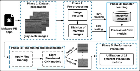
1.1 The Problem

Malware (malicious software) is software designed to damage systems or steal information. Security researchers need to classify malware into families - groups of malware that behave similarly or come from the same source. This helps understand threats and build defenses.

The traditional way to classify malware is manual analysis. You’d open the malware binary in specialized tools, reverse engineer it to see what it does, watch how it behaves when running, and compare it to known families. This can take hours or even days per sample. When you’re dealing with thousands of new malware samples every day, manual analysis doesn’t scale.

This is where machine learning can help. If we can teach a computer to recognize patterns that distinguish different malware families, we can automate most of the classification work.

1.2 Why Use Images?

Here’s the interesting part - instead of feeding raw binary code to our model, we convert malware binaries into grayscale images. This might sound weird, but there’s good reasoning:

1. Safety: We’re working with images of malware, not actual executable code. You can’t accidentally infect your computer with a picture.
2. Visual patterns: Malware from the same family often has similar code structure, which shows up as visual patterns in images.
3. No need to understand assembly: The model looks at pixel patterns rather than trying to understand machine code.

The conversion is simple. A binary file is just a sequence of bytes (values from 0 to 255). We map each byte to a pixel where the byte value determines the pixel’s brightness. Byte value 0 becomes black, 255 becomes white, and everything in between is a shade of gray.

Figure 1: Binary to image conversion diagram - each byte maps to one pixel

1.3 Our Approach

We’ll build a classifier using a Convolutional Neural Network (CNN). Don’t worry if you haven’t heard of CNNs - I’ll explain them when we get there. For now, think of it as a type of model that’s really good at recognizing patterns in images.

The workflow is:

1. Get a dataset of malware images (already converted from binaries)
2. Split it into training and testing sets
3. Train a CNN to recognize which family each image belongs to
4. Test how accurate our classifier is

---

Python & Machine Learning: From Absolute Zero

This guide assumes you know basic programming (variables, loops, functions) but nothing about Python or machine learning. We’ll build up from first principles.

Setting Up Python

What is Python? It’s a programming language. Unlike compiled languages (C, C++), Python runs line-by-line through an interpreter. This makes it slower for raw computation but way faster for development.

Installing Python:

1. Download Python 3.8+ from python.org (or use Anaconda, which bundles everything)
2. During install, check “Add Python to PATH”
3. Verify: open terminal/command prompt, type python --version

Installing libraries:

pip install numpy pandas torch torchvision matplotlib

pip is Python’s package installer. It downloads libraries from the internet and sets them up.

What’s a virtual environment? (Optional but recommended)

python -m venv ml_env
# Activate it:
# Windows: ml_env\Scripts\activate
# Mac/Linux: source ml_env/bin/activate

This creates an isolated Python setup. Libraries you install here won’t mess with other projects. When you’re done, type deactivate.

Python Basics You Need

Variables - no types needed:

x = 5              # integer
y = 3.14           # float
name = "malware"   # string
is_packed = True   # boolean

Python figures out types automatically. No need to write int x = 5; like in C.

Lists - ordered collections:

files = ["sample1.exe", "sample2.exe", "sample3.exe"]
print(files[0])  # sample1.exe (indexing starts at 0)
files.append("sample4.exe")  # add to end

Dictionaries - key-value pairs:

labels = {
    "sample1.exe": "trojan",
    "sample2.exe": "ransomware",
    "sample3.exe": "trojan"
}
print(labels["sample1.exe"])  # trojan

Loops:

# Loop through list
for file in files:
    print(file)

# Loop with index
for i in range(10):  # 0 to 9
    print(i)

Functions:

def classify_file(filename):
    # do something
    return result

output = classify_file("sample.exe")

Importing libraries:

import numpy as np  # import and give it a short name
from torch import nn  # import specific part

# Now use them:
array = np.array([1, 2, 3])
layer = nn.Linear(10, 5)

Understanding Arrays (NumPy)

Why arrays matter: In machine learning, everything is numbers in grids. An image? Numbers in a grid. Model weights? Numbers in a grid. Arrays are how we store and manipulate these grids efficiently.

Creating arrays:

import numpy as np

# From a list
arr = np.array([1, 2, 3, 4, 5])
print(arr.shape)  # (5,) - one dimension, 5 elements

# 2D array (matrix)
matrix = np.array([
    [1, 2, 3],
    [4, 5, 6]
])
print(matrix.shape)  # (2, 3) - 2 rows, 3 columns

Shape is crucial. It tells you dimensions. A color image that’s 256x256 pixels has shape (256, 256, 3) - height, width, color channels (red, green, blue).

Array operations:

a = np.array([1, 2, 3])
b = np.array([4, 5, 6])

# Element-wise operations (happens to each pair)
print(a + b)  # [5, 7, 9]
print(a * 2)  # [2, 4, 6]
print(a * b)  # [4, 10, 18] - element by element

# Useful functions
print(a.mean())  # average: 2.0
print(a.max())   # maximum: 3
print(a.sum())   # sum: 6

Why is this faster than Python lists? NumPy arrays are stored in continuous memory blocks and operations are implemented in C. A loop in pure Python is slow. A NumPy operation runs compiled C code.

# Slow way (pure Python)
result = []
for i in range(1000000):
    result.append(i * 2)

# Fast way (NumPy)
result = np.arange(1000000) * 2  # 10-100x faster

Indexing and slicing:

arr = np.array([10, 20, 30, 40, 50])

print(arr[0])      # 10 - first element
print(arr[-1])     # 50 - last element
print(arr[1:4])    # [20, 30, 40] - elements 1,2,3 (4 is excluded)
print(arr[:3])     # [10, 20, 30] - first three
print(arr[2:])     # [30, 40, 50] - from index 2 to end

# 2D slicing
matrix = np.array([
    [1, 2, 3],
    [4, 5, 6],
    [7, 8, 9]
])
print(matrix[0, :])    # [1, 2, 3] - first row, all columns
print(matrix[:, 0])    # [1, 4, 7] - all rows, first column
print(matrix[1, 2])    # 6 - row 1, column 2

Reshaping:

arr = np.array([1, 2, 3, 4, 5, 6])
matrix = arr.reshape(2, 3)  # 2 rows, 3 columns
# [[1, 2, 3],
#  [4, 5, 6]]

# Flatten back
flat = matrix.reshape(-1)  # -1 means "figure it out"
# [1, 2, 3, 4, 5, 6]

When loading images for ML, you’ll constantly reshape: from (height, width, channels) to (channels, height, width) and back.

What is Machine Learning, Actually?

The problem: You have data (malware samples) and labels (which family each belongs to). You want a function that maps data to labels.

The old way: Write rules by hand.

def classify(file):
    if "ransomware_string" in file:
        return "ransomware"
    elif file_size > 5MB and has_encryption:
        return "trojan"
    # ... hundreds of rules

This breaks with new malware. Rules don’t adapt.

The ML way: Learn the function from examples.

1. Show the computer 10,000 labeled malware samples
2. It finds patterns automatically
3. Test on new samples it’s never seen

How does learning work?

Imagine teaching a kid to recognize cats vs dogs:

• Show picture: “This is a cat”
• Kid guesses: “Dog!”
• Correct them: “No, cat. Look at the ears, they’re pointy”
• Kid adjusts their understanding
• Repeat with thousands of pictures
• Eventually kid learns: pointy ears + small nose + certain body shape = cat

ML does the same, but with math instead of words.

Neural Networks - The Math Function

What’s a neural network? It’s a mathematical function with adjustable parameters (called weights).

Simple example:

output = weight * input + bias

If input = 5, weight = 2, bias = 3:

output = 2 * 5 + 3 = 13

That’s a neural network with one weight and one bias. Useless for real problems, but it’s the core idea.

Making it useful: Stack many of these together in layers.

# Layer 1
hidden = weight1 * input + bias1

# Layer 2  
output = weight2 * hidden + bias2

With enough layers and weights, you can approximate any function. This is why deep learning works.

Real neural network in PyTorch:

import torch
import torch.nn as nn

# Define network structure
class SimpleNet(nn.Module):
    def __init__(self):
        super().__init__()
        self.layer1 = nn.Linear(10, 20)  # 10 inputs -> 20 outputs
        self.layer2 = nn.Linear(20, 5)   # 20 inputs -> 5 outputs
    
    def forward(self, x):
        x = self.layer1(x)
        x = torch.relu(x)  # activation (explained below)
        x = self.layer2(x)
        return x

# Create the network
model = SimpleNet()

What does nn.Linear(10, 20) do?

It creates a layer with 10 inputs and 20 outputs. Internally, it has:

• A weight matrix of shape (20, 10) - 200 numbers
• A bias vector of shape (20) - 20 numbers

When you pass data through:

output = layer(input)

It computes: output = input @ weights + bias (matrix multiplication plus bias)

Activation functions - why ReLU?

Without activation functions, stacking layers is pointless. Here’s why:

# Two linear layers without activation
hidden = weight1 * input + bias1
output = weight2 * hidden + bias2

# Substitute:
output = weight2 * (weight1 * input + bias1) + bias2
output = (weight2 * weight1) * input + (weight2 * bias1 + bias2)

You can collapse it to one layer. Multiple layers don’t add power.

With activation (non-linearity):

hidden = relu(weight1 * input + bias1)
output = weight2 * hidden + bias2

Now you can’t collapse it. The relu function introduces non-linearity.

What’s ReLU?

def relu(x):
    return max(0, x)  # if x < 0, return 0, else return x

Simple but effective. Negative values become zero, positive values pass through.

relu(-5) = 0
relu(3) = 3
relu(0) = 0

Other activations exist (sigmoid, tanh), but ReLU is standard because it’s fast and works well.

Training - How Learning Happens

The training loop (conceptual):

1. Forward pass: Put data through the network, get predictions
2. Calculate loss: How wrong are the predictions?
3. Backward pass: Calculate how to adjust weights to reduce loss
4. Update weights: Make small adjustments
5. Repeat: Do this thousands of times

Loss function: Measures error. If your network predicts 0.8 for “ransomware” but the real answer is 1.0, the loss captures that 0.2 gap.

Common loss for classification: Cross-Entropy Loss

criterion = nn.CrossEntropyLoss()
loss = criterion(predictions, true_labels)

The loss is a single number. Higher = worse predictions.

Backward pass (backpropagation): This is where calculus happens. Given the loss, PyTorch calculates gradients - how much each weight contributed to the error.

You don’t compute derivatives by hand. PyTorch does it automatically:

loss.backward()  # calculates gradients for all weights

Optimizer: Updates weights based on gradients.

optimizer = torch.optim.Adam(model.parameters(), lr=0.001)

# After loss.backward()
optimizer.step()  # adjusts weights

lr=0.001 is the learning rate - how big each step is. Too large and training is unstable. Too small and learning is slow.

Full training loop:

model = SimpleNet()
criterion = nn.CrossEntropyLoss()
optimizer = torch.optim.Adam(model.parameters(), lr=0.001)

for epoch in range(10):  # train for 10 epochs
    for inputs, labels in data_loader:  # go through all data
        # Forward pass
        predictions = model(inputs)
        loss = criterion(predictions, labels)
        
        # Backward pass
        optimizer.zero_grad()  # reset gradients
        loss.backward()        # calculate gradients
        optimizer.step()       # update weights
        
    print(f"Epoch {epoch}, Loss: {loss.item()}")

What’s an epoch? One pass through the entire dataset. If you have 10,000 samples, one epoch means showing all 10,000 to the model.

What’s a batch? Instead of processing one sample at a time, you group samples. A batch of 32 means processing 32 samples together. This is faster on GPUs.

# If dataset has 10,000 samples and batch_size=32
# One epoch = 10,000/32 = 313 batches

Convolutional Neural Networks (CNNs)

The problem with regular networks for images:

A 256x256 RGB image has 256 × 256 × 3 = 196,608 pixels. If your first layer is nn.Linear(196608, 1000), you need 196 million weights for just the first layer. That’s:

• Extremely slow to train
• Requires massive memory
• Will overfit (memorize training data, fail on new data)

How CNNs solve this:

Instead of connecting every pixel to every neuron, use convolutional filters - small sliding windows that scan the image.

What’s a convolution?

Imagine a 3x3 magnifying glass scanning across an image:

Image:          Filter:
[1 2 3 4 5]     [1 0 -1]
[6 7 8 9 0]     [1 0 -1]
[1 2 3 4 5]     [1 0 -1]

Place filter on top-left:
1*1 + 2*0 + 3*(-1) +
6*1 + 7*0 + 8*(-1) +
1*1 + 2*0 + 3*(-1) = -10

Slide right one pixel, repeat...

One filter produces one output map. Use 64 filters and you get 64 output maps.

In PyTorch:

conv = nn.Conv2d(
    in_channels=3,   # RGB input
    out_channels=64, # 64 filters
    kernel_size=3,   # 3x3 filters
    padding=1        # keep same size
)

# Input: (batch, 3, 256, 256)
# Output: (batch, 64, 256, 256)

Each of the 64 filters learns to detect a different pattern. First layer might learn:

• Vertical edges
• Horizontal edges
• Diagonal lines
• Color gradients

Pooling - reducing size:

After convolution, use pooling to shrink the image. Max pooling takes the maximum value in each 2x2 region:

Input:          Output (2x2 max pool):
[1 3 2 4]       [3 4]
[5 2 8 1]       
              →  [5 8]
[2 1 3 6]
[4 2 7 3]

This reduces 4x4 to 2x2. Reduces computation and makes the network focus on “is this feature present?” rather than “exactly where is it?”

pool = nn.MaxPool2d(kernel_size=2, stride=2)

# Input: (batch, 64, 256, 256)
# Output: (batch, 64, 128, 128)

Typical CNN architecture:

class CNN(nn.Module):
    def __init__(self):
        super().__init__()
        self.conv1 = nn.Conv2d(3, 64, kernel_size=3, padding=1)
        self.pool1 = nn.MaxPool2d(2, 2)
        
        self.conv2 = nn.Conv2d(64, 128, kernel_size=3, padding=1)
        self.pool2 = nn.MaxPool2d(2, 2)
        
        self.conv3 = nn.Conv2d(128, 256, kernel_size=3, padding=1)
        self.pool3 = nn.MaxPool2d(2, 2)
        
        # After 3 pooling layers, 256x256 becomes 32x32
        self.fc1 = nn.Linear(256 * 32 * 32, 512)
        self.fc2 = nn.Linear(512, 10)  # 10 classes
    
    def forward(self, x):
        # Input: (batch, 3, 256, 256)
        x = torch.relu(self.conv1(x))  # (batch, 64, 256, 256)
        x = self.pool1(x)              # (batch, 64, 128, 128)
        
        x = torch.relu(self.conv2(x))  # (batch, 128, 128, 128)
        x = self.pool2(x)              # (batch, 128, 64, 64)
        
        x = torch.relu(self.conv3(x))  # (batch, 256, 64, 64)
        x = self.pool3(x)              # (batch, 256, 32, 32)
        
        # Flatten for fully connected layers
        x = x.view(x.size(0), -1)      # (batch, 256*32*32)
        x = torch.relu(self.fc1(x))    # (batch, 512)
        x = self.fc2(x)                # (batch, 10)
        return x

Why this works for malware images:

When you convert a malware binary to an image:

• Similar malware families use similar code structures
• Packers leave visual signatures (high entropy regions look different from normal code)
• API call sequences create recognizable patterns
• Code sections (.text, .data, .rsrc) have distinct visual features

The CNN learns these patterns layer by layer:

• Layer 1: Detects basic byte patterns, edges, gradients
• Layer 2: Combines into code structures, data patterns
• Layer 3: Recognizes “this looks like UPX packer” or “this is Emotet’s signature”

The model doesn’t “understand” what a packer is. It just learns: “samples with these visual features are usually labeled ‘trojan’, so I’ll predict ‘trojan’.”

Putting It Together - Loading Data

Your dataset structure:

data/
  train/
    trojan/
      sample1.png
      sample2.png
    ransomware/
      sample3.png
      sample4.png
  test/
    trojan/
      sample5.png
    ransomware/
      sample6.png

Loading with torchvision:

from torchvision import datasets, transforms
from torch.utils.data import DataLoader

# Define transformations
transform = transforms.Compose([
    transforms.Resize((256, 256)),      # resize to 256x256
    transforms.ToTensor(),              # convert to tensor, scale 0-1
    transforms.Normalize(               # standardize
        mean=[0.5, 0.5, 0.5],
        std=[0.5, 0.5, 0.5]
    )
])

# Load dataset
train_dataset = datasets.ImageFolder(
    root='data/train',
    transform=transform
)

# Create data loader
train_loader = DataLoader(
    train_dataset,
    batch_size=32,
    shuffle=True  # randomize order
)

# Use in training
for images, labels in train_loader:
    # images: (32, 3, 256, 256) - batch of 32 RGB images
    # labels: (32,) - batch of 32 labels
    predictions = model(images)
    loss = criterion(predictions, labels)
    # ... backward pass, etc.

What does each transformation do?

• Resize(256, 256): Makes all images the same size (neural networks need fixed input size)
• ToTensor(): Converts PIL Image (0-255) to PyTorch tensor (0.0-1.0)
• Normalize(): Shifts values to have mean 0, std 1 (helps training converge faster)

GPU Acceleration

Why GPU? Matrix multiplication is what takes time in neural networks. GPUs have thousands of cores designed for parallel math. A 10-hour training run on CPU takes 30 minutes on GPU.

Using GPU in PyTorch:

# Check if GPU available
device = torch.device("cuda" if torch.cuda.is_available() else "cpu")
print(f"Using {device}")

# Move model to GPU
model = model.to(device)

# Move data to GPU in training loop
for images, labels in train_loader:
    images = images.to(device)
    labels = labels.to(device)
    
    predictions = model(images)
    loss = criterion(predictions, labels)
    # ... rest of training

That’s it. .to(device) handles everything.

Evaluation - Did It Work?

Accuracy:

correct = 0
total = 0

model.eval()  # set to evaluation mode (turns off dropout, etc.)
with torch.no_grad():  # don't calculate gradients
    for images, labels in test_loader:
        images = images.to(device)
        labels = labels.to(device)
        
        outputs = model(images)
        _, predicted = torch.max(outputs, 1)
        
        total += labels.size(0)
        correct += (predicted == labels).sum().item()

accuracy = 100 * correct / total
print(f"Accuracy: {accuracy}%")

What’s torch.max(outputs, 1)?

Model outputs logits (raw scores) for each class. If you have 10 classes, output shape is (batch, 10).

# Example output for one sample:
outputs = [2.3, 0.1, -1.5, 4.2, 0.8, ...]
          # class 0, 1, 2, 3, 4, ...

# torch.max finds highest value
_, predicted = torch.max(outputs, 1)
# predicted = 3 (class 3 has highest score: 4.2)

Confusion matrix - see which mistakes:

from sklearn.metrics import confusion_matrix
import matplotlib.pyplot as plt
import numpy as np

# Collect all predictions and true labels
all_preds = []
all_labels = []

model.eval()
with torch.no_grad():
    for images, labels in test_loader:
        images = images.to(device)
        outputs = model(images)
        _, preds = torch.max(outputs, 1)
        
        all_preds.extend(preds.cpu().numpy())
        all_labels.extend(labels.cpu().numpy())

# Compute confusion matrix
cm = confusion_matrix(all_labels, all_preds)

# Plot
plt.imshow(cm, cmap='Blues')
plt.colorbar()
plt.xlabel('Predicted')
plt.ylabel('True')
plt.title('Confusion Matrix')
plt.show()

The diagonal shows correct predictions. Off-diagonal shows which classes get confused.

Common Issues and Debugging

Model outputs NaN (Not a Number):

• Learning rate too high, reduce it
• Check for division by zero
• Check for log(0) or sqrt(negative)

Loss not decreasing:

• Learning rate too low
• Bug in model (check shapes)
• Data not normalized
• Try on a tiny subset first (overfit 10 samples to verify code works)

Overfitting (train accuracy high, test accuracy low):

• Model too complex, reduce layers or neurons
• Add dropout: nn.Dropout(0.5) randomly zeros 50% of neurons during training
• Get more data
• Add data augmentation (rotate, flip images)

Out of memory:

• Reduce batch size
• Reduce image size
• Use smaller model
• Use gradient accumulation (update every N batches instead of every batch)

Check tensor shapes:

print(x.shape)  # always print shapes when debugging

90% of bugs are shape mismatches.

---

3. The Dataset

3.1 Dataset Overview

We’ll use the malimg dataset. It contains 9,339 grayscale images representing 25 different malware families. You can download it from Kaggle.

Each image is a visualization of a Windows executable (PE file). The dataset is organized into folders where each folder name is the malware family name.

Figure 2: Example malware image showing byte patterns

3.2 Understanding Class Distribution

Before training, it’s important to know if some classes are over-represented. If 90% of our data is from one family, the model might just learn to guess that family every time.

Let’s explore the dataset. This code counts how many images are in each family folder:

import os
import matplotlib.pyplot as plt
import seaborn as sns

# Point to where you unzipped the dataset
DATA_BASE_PATH = "./malimg_paper_dataset_imgs/"

# Count images in each family folder
dist = {}
for family_name in os.listdir(DATA_BASE_PATH):
    family_folder = os.path.join(DATA_BASE_PATH, family_name)
    # Count files in this folder
    dist[family_name] = len(os.listdir(family_folder))

# Print what we found
print(f"Total families: {len(dist)}")
print(f"Total images: {sum(dist.values())}")

Now let’s visualize this:

# Prepare data for plotting
families = list(dist.keys())
counts = list(dist.values())

# Create the plot
plt.figure(figsize=(10, 8))
sns.barplot(y=families, x=counts, orient='h')
plt.title("Malware Family Distribution")
plt.xlabel("Number of Samples")
plt.ylabel("Malware Family")
plt.tight_layout()
plt.show()

Figure 3: Class distribution bar chart - Allaple.A and Allaple.L have the most samples

From the plot, we can see the dataset is imbalanced. Some families have thousands of samples while others have just a few hundred. This is common in real-world datasets. Our model might perform better on families with more training examples.

3.3 Visual Patterns in Malware Families

Let’s look at two samples from the same family to see if they really share visual patterns:

Figure 4: Two FakeRean samples side by side showing similar vertical striping patterns

You can see both images have similar structures. These patterns come from shared code, data layouts, or packing methods used by this malware family. The CNN will learn to recognize these patterns.

---

4. Complete Pipeline: From Data to Trained Model

Now let’s build the complete pipeline. This is one continuous program that goes from loading data to training a classifier. I’ll explain each part as we go.

4.1 Setup and Imports

First, import everything we need:

import os
import time
import torch
import torch.nn as nn
import torch.optim as optim
from torch.utils.data import DataLoader
from torchvision import transforms, datasets, models
import matplotlib.pyplot as plt

# Check if GPU is available - training is much faster on GPU
device = torch.device("cuda" if torch.cuda.is_available() else "cpu")
print(f"Using device: {device}")

The device variable tells PyTorch whether to use a GPU or CPU. If you have a NVIDIA GPU with CUDA installed, training will be much faster.

4.2 Step 1: Preparing the Data

First, we need to split our dataset into training and testing sets. We’ll use 80% for training and 20% for testing.

# Install split-folders if you haven't: pip install split-folders
import splitfolders

# Where your original dataset is
INPUT_PATH = "./malimg_paper_dataset_imgs/"
# Where to save the split data
OUTPUT_PATH = "./data_split/"

# Split: 80% train, 0% validation, 20% test
# We're not using validation here to keep it simple
splitfolders.ratio(
    input=INPUT_PATH, 
    output=OUTPUT_PATH,
    seed=42,  # Random seed for reproducibility
    ratio=(0.8, 0, 0.2)
)
print("Dataset split complete!")

Why split the data? If we test on the same data we trained on, the model might just memorize the training examples. Testing on unseen data tells us if the model actually learned patterns or just memorized.

4.3 Step 2: Image Preprocessing

CNNs need consistent input. All images must be the same size, and pixel values should be normalized.

# Define how we'll preprocess images
transform = transforms.Compose([
    # Resize all images to 75x75 pixels
    # Why 75x75? Smaller = faster training, but we lose some detail
    # This is a balance between speed and information
    transforms.Resize((75, 75)),
    
    # Convert PIL Image to PyTorch tensor (multi-dimensional array)
    # Also scales pixel values from 0-255 to 0-1
    transforms.ToTensor(),
    
    # Normalize using ImageNet statistics
    # These values are standard for models pre-trained on ImageNet
    # Normalization helps the model train more stably
    transforms.Normalize(
        mean=[0.485, 0.456, 0.406],  # Average RGB values
        std=[0.229, 0.224, 0.225]     # Standard deviations
    )
])

Why normalize? Neural networks train better when inputs are in a consistent range. Without normalization, some features might dominate just because they have larger numbers, not because they’re more important.

Why these specific mean/std values? We’re using a pre-trained model (explained later) that was trained with these normalization values. Using the same preprocessing ensures consistency.

Now let’s load the datasets:

# Load training data
# ImageFolder expects data organized as: root/class_name/image.png
train_dataset = datasets.ImageFolder(
    root=os.path.join(OUTPUT_PATH, "train"),
    transform=transform
)

# Load test data
test_dataset = datasets.ImageFolder(
    root=os.path.join(OUTPUT_PATH, "test"),
    transform=transform
)

# How many classes do we have?
num_classes = len(train_dataset.classes)
print(f"Number of malware families: {num_classes}")
print(f"Training samples: {len(train_dataset)}")
print(f"Test samples: {len(test_dataset)}")

4.4 Step 3: Creating Data Loaders

Data loaders handle batching and shuffling. Instead of feeding one image at a time, we feed batches (groups of images). This is more efficient and helps the model learn better.

# Batch size: how many images to process together
# Larger batches = faster but need more memory
# 32-128 is typical for image classification
BATCH_SIZE = 64

# Create loader for training data
train_loader = DataLoader(
    train_dataset,
    batch_size=BATCH_SIZE,
    shuffle=True,        # Randomize order each epoch
    num_workers=2,       # Parallel data loading (faster)
    pin_memory=True      # Faster GPU transfer
)

# Create loader for test data
test_loader = DataLoader(
    test_dataset,
    batch_size=BATCH_SIZE,
    shuffle=False,       # No need to shuffle test data
    num_workers=2,
    pin_memory=True
)

Why shuffle training data? If we always see malware families in the same order, the model might learn order-dependent patterns instead of real distinguishing features. Shuffling prevents this.

Why not shuffle test data? Order doesn’t matter for testing - we just want consistent results.

Let’s check what a batch looks like:

# Get one batch
images, labels = next(iter(train_loader))
print(f"Batch shape: {images.shape}")  # Should be [batch_size, 3, 75, 75]
print(f"Labels shape: {labels.shape}") # Should be [batch_size]

# Note: images has 3 channels even though our images are grayscale
# This is because transforms.ToTensor() converts grayscale to RGB format
# (duplicating the single channel three times) to match the pre-trained model's expectations

4.5 Step 4: Building the Model

Now the interesting part. We’ll use transfer learning - starting with a model pre-trained on a huge dataset (ImageNet) and adapting it for our task.

Why transfer learning? Training a CNN from scratch requires millions of images and days of computation. By starting with a pre-trained model, we leverage knowledge it already learned about recognizing patterns in images.

class MalwareClassifier(nn.Module):
    def __init__(self, num_classes):
        super(MalwareClassifier, self).__init__()
        
        # Load ResNet50 with pre-trained weights
        # ResNet50 is a 50-layer CNN that's proven to work well
        self.resnet = models.resnet50(weights='DEFAULT')
        
        # Freeze all layers except the last one
        # "Freezing" means these weights won't change during training
        # Why? These layers already learned useful low-level features
        # (edges, textures, shapes) from ImageNet
        # Only the final layer needs to adapt to malware classification
        for param in self.resnet.parameters():
            param.requires_grad = False
        
        # Replace the final layer
        # Original ResNet50 outputs 1000 classes (ImageNet has 1000 categories)
        # We need to output num_classes (25 malware families)
        num_features = self.resnet.fc.in_features  # Usually 2048
        
        self.resnet.fc = nn.Sequential(
            nn.Linear(num_features, 512),  # Intermediate layer
            nn.ReLU(),                      # Activation function
            nn.Dropout(0.3),                # Randomly drop 30% of connections
                                            # This prevents overfitting
            nn.Linear(512, num_classes)     # Final output layer
        )

    def forward(self, x):
        # This defines how data flows through the model
        return self.resnet(x)

# Create the model
model = MalwareClassifier(num_classes)
model = model.to(device)  # Move model to GPU if available

print(f"Model created with {num_classes} output classes")

Why freeze layers? Training all 50 layers would take much longer and might actually perform worse with our small dataset. The early layers learn generic features (edges, textures) that are useful for any image task. We only need to teach the final layers what patterns identify each malware family.

What’s Dropout? During training, dropout randomly “turns off” some neurons. This forces the network to learn robust features rather than memorizing specific examples.

4.6 Step 5: Training Setup

Before training, we define:

• Loss function: Measures how wrong the model’s predictions are
• Optimizer: Algorithm that adjusts weights to reduce loss
• Learning rate: How big each adjustment step should be

# Loss function for multi-class classification
# CrossEntropyLoss combines softmax and negative log-likelihood
# It's standard for classification tasks
criterion = nn.CrossEntropyLoss()

# Optimizer: Adam is usually a good default choice
# It adapts the learning rate automatically during training
optimizer = optim.Adam(
    model.resnet.fc.parameters(),  # Only train the final layer
    lr=0.001  # Learning rate - how fast we update weights
              # 0.001 is a common starting point
)

# Learning rate scheduler (optional but helpful)
# Reduces learning rate when progress plateaus
# This helps fine-tune the model in later epochs
scheduler = optim.lr_scheduler.ReduceLROnPlateau(
    optimizer,
    mode='max',      # We want to maximize accuracy
    factor=0.5,      # Reduce LR by half when needed
    patience=2,      # Wait 2 epochs before reducing
    verbose=True
)

What’s a learning rate? If loss is a valley and we want to reach the bottom, learning rate is our step size. Too large and we overshoot. Too small and training takes forever. We start at 0.001 and reduce it if we stop improving.

4.7 Step 6: The Training Loop

This is where the actual learning happens. For each epoch (one pass through all training data):

1. Feed batches of images to the model
2. Calculate how wrong the predictions are (loss)
3. Adjust weights to reduce the error (backpropagation)
4. Repeat

def train_one_epoch(model, train_loader, criterion, optimizer, device):
    """Train for one epoch and return average loss and accuracy"""
    model.train()  # Set model to training mode (enables dropout, etc.)
    
    running_loss = 0.0
    correct = 0
    total = 0
    
    for batch_idx, (images, labels) in enumerate(train_loader):
        # Move data to GPU if available
        images = images.to(device)
        labels = labels.to(device)
        
        # Zero the gradients from previous batch
        # (PyTorch accumulates gradients by default)
        optimizer.zero_grad()
        
        # Forward pass: get model predictions
        outputs = model(images)
        
        # Calculate loss (how wrong are we?)
        loss = criterion(outputs, labels)
        
        # Backward pass: compute gradients
        # This calculates how much each weight contributed to the error
        loss.backward()
        
        # Update weights based on gradients
        optimizer.step()
        
        # Track statistics
        running_loss += loss.item()
        _, predicted = outputs.max(1)  # Get class with highest score
        total += labels.size(0)
        correct += predicted.eq(labels).sum().item()
        
        # Print progress every 20 batches
        if (batch_idx + 1) % 20 == 0:
            print(f"  Batch {batch_idx+1}/{len(train_loader)}, "
                  f"Loss: {loss.item():.4f}")
    
    # Calculate averages for the epoch
    avg_loss = running_loss / len(train_loader)
    accuracy = 100.0 * correct / total
    
    return avg_loss, accuracy

What’s backpropagation? It’s the algorithm that figures out how to adjust each weight. Starting from the output error, it works backwards through the network calculating each weight’s contribution to the mistake.

4.8 Step 7: Evaluation Function

We need to check how well the model performs on test data:

def evaluate(model, test_loader, criterion, device):
    """Evaluate model on test data"""
    model.eval()  # Set to evaluation mode (disables dropout)
    
    running_loss = 0.0
    correct = 0
    total = 0
    
    # Don't calculate gradients during testing (saves memory and time)
    with torch.no_grad():
        for images, labels in test_loader:
            images = images.to(device)
            labels = labels.to(device)
            
            # Get predictions
            outputs = model(images)
            loss = criterion(outputs, labels)
            
            # Track statistics
            running_loss += loss.item()
            _, predicted = outputs.max(1)
            total += labels.size(0)
            correct += predicted.eq(labels).sum().item()
    
    avg_loss = running_loss / len(test_loader)
    accuracy = 100.0 * correct / total
    
    return avg_loss, accuracy

4.9 Step 8: Main Training Loop

Now we put it all together:

# Training parameters
NUM_EPOCHS = 10  # How many times to go through the entire dataset

# Track progress
train_losses = []
train_accuracies = []
test_losses = []
test_accuracies = []

print("Starting training...")
best_test_acc = 0.0

for epoch in range(NUM_EPOCHS):
    print(f"\nEpoch {epoch+1}/{NUM_EPOCHS}")
    print("-" * 50)
    
    # Train for one epoch
    train_loss, train_acc = train_one_epoch(
        model, train_loader, criterion, optimizer, device
    )
    
    # Evaluate on test set
    test_loss, test_acc = evaluate(
        model, test_loader, criterion, device
    )
    
    # Update learning rate based on test accuracy
    scheduler.step(test_acc)
    
    # Save statistics
    train_losses.append(train_loss)
    train_accuracies.append(train_acc)
    test_losses.append(test_loss)
    test_accuracies.append(test_acc)
    
    # Print epoch summary
    print(f"\nEpoch {epoch+1} Summary:")
    print(f"  Train Loss: {train_loss:.4f}, Train Acc: {train_acc:.2f}%")
    print(f"  Test Loss: {test_loss:.4f}, Test Acc: {test_acc:.2f}%")
    
    # Save best model
    if test_acc > best_test_acc:
        best_test_acc = test_acc
        torch.save(model.state_dict(), 'best_malware_classifier.pth')
        print(f"  *** New best test accuracy! Model saved. ***")

print("\nTraining complete!")
print(f"Best test accuracy: {best_test_acc:.2f}%")

Why save the best model? Test accuracy might fluctuate. We save the version that performed best so we don’t lose it if later epochs perform worse.

4.10 Step 9: Visualizing Training Progress

Let’s see how the model improved over time:

# Create two plots side by side
fig, (ax1, ax2) = plt.subplots(1, 2, figsize=(14, 5))

# Plot 1: Loss over time
ax1.plot(train_losses, label='Training Loss', marker='o')
ax1.plot(test_losses, label='Test Loss', marker='s')
ax1.set_xlabel('Epoch')
ax1.set_ylabel('Loss')
ax1.set_title('Loss Over Time')
ax1.legend()
ax1.grid(True, alpha=0.3)

# Plot 2: Accuracy over time
ax2.plot(train_accuracies, label='Training Accuracy', marker='o')
ax2.plot(test_accuracies, label='Test Accuracy', marker='s')
ax2.set_xlabel('Epoch')
ax2.set_ylabel('Accuracy (%)')
ax2.set_title('Accuracy Over Time')
ax2.legend()
ax2.grid(True, alpha=0.3)

plt.tight_layout()
plt.savefig('training_progress.png', dpi=150, bbox_inches='tight')
plt.show()

print("Training curves saved as 'training_progress.png'")

Figure 5: Training accuracy graph showing steady increase over epochs

What to look for:

• Training accuracy should increase (loss should decrease)
• If test accuracy is much lower than training, we’re overfitting
• If both are low, the model isn’t learning well (might need more training or a different architecture)

4.11 Step 10: Testing the Model

Let’s test our trained model on a few specific examples:

def predict_sample(model, image_path, transform, device, class_names):
    """Predict the malware family for a single image"""
    from PIL import Image
    
    model.eval()
    
    # Load and preprocess the image
    image = Image.open(image_path).convert('RGB')
    image_tensor = transform(image).unsqueeze(0)  # Add batch dimension
    image_tensor = image_tensor.to(device)
    
    # Get prediction
    with torch.no_grad():
        output = model(image_tensor)
        probabilities = torch.nn.functional.softmax(output, dim=1)
        confidence, predicted_class = probabilities.max(1)
    
    predicted_family = class_names[predicted_class.item()]
    confidence_pct = confidence.item() * 100
    
    return predicted_family, confidence_pct

# Get class names from the dataset
class_names = train_dataset.classes

# Test on a random image from test set
import random
test_image_path = random.choice(test_dataset.imgs)[0]
actual_family = os.path.basename(os.path.dirname(test_image_path))

predicted_family, confidence = predict_sample(
    model, test_image_path, transform, device, class_names
)

print(f"\nTest Image: {test_image_path}")
print(f"Actual Family: {actual_family}")
print(f"Predicted Family: {predicted_family}")
print(f"Confidence: {confidence:.2f}%")
print(f"Correct: {actual_family == predicted_family}")

---

5. Understanding the Results

5.1 Typical Performance

With this setup, you should see:

• Training accuracy reaching 95-97% after 10 epochs
• Test accuracy around 85-90%
• The gap between training and test accuracy indicates some overfitting, which is normal with a small dataset

5.2 What Each Metric Means

When evaluating classifiers, we look at several metrics:

Accuracy: Percentage of correct predictions

Accuracy = (Correct Predictions) / (Total Predictions)

This is intuitive but can be misleading with imbalanced data. If 95% of samples are from one family, you could get 95% accuracy just by always guessing that family.

Precision: Of all predictions for a specific family, how many were correct?

Precision = (True Positives) / (True Positives + False Positives)

High precision means when the model says “this is family X”, it’s usually right.

Recall: Of all actual samples from a family, how many did we correctly identify?

Recall = (True Positives) / (True Positives + False Negatives)

High recall means we catch most instances of each family.

F1-Score: Harmonic mean of precision and recall

F1 = 2 × (Precision × Recall) / (Precision + Recall)

F1-score is useful when you care about both false positives and false negatives equally.

5.3 Computing Detailed Metrics

Let’s calculate per-class metrics:

from sklearn.metrics import classification_report, confusion_matrix
import numpy as np

def detailed_evaluation(model, test_loader, device, class_names):
    """Get detailed per-class metrics"""
    model.eval()
    
    all_predictions = []
    all_labels = []
    
    with torch.no_grad():
        for images, labels in test_loader:
            images = images.to(device)
            outputs = model(images)
            _, predicted = outputs.max(1)
            
            all_predictions.extend(predicted.cpu().numpy())
            all_labels.extend(labels.numpy())
    
    # Generate classification report
    print("\nDetailed Classification Report:")
    print("=" * 70)
    report = classification_report(
        all_labels, 
        all_predictions, 
        target_names=class_names,
        digits=3
    )
    print(report)
    
    # Confusion matrix
    cm = confusion_matrix(all_labels, all_predictions)
    return cm

# Run detailed evaluation
cm = detailed_evaluation(model, test_loader, device, class_names)

# Find which families the model struggles with
print("\nFamilies with lowest accuracy:")
class_accuracies = cm.diagonal() / cm.sum(axis=1)
worst_families = np.argsort(class_accuracies)[:5]

for idx in worst_families:
    family = class_names[idx]
    acc = class_accuracies[idx] * 100
    samples = cm.sum(axis=1)[idx]
    print(f"  {family}: {acc:.1f}% ({samples} test samples)")

5.4 Why Some Families Perform Poorly

You’ll notice some families have lower accuracy. Common reasons:

1. Small sample size: Families with few training examples are harder to learn
2. Visual similarity: Some families might look very similar to each other
3. Class imbalance: The model sees more examples from large families, so it learns those better

---

6. Improving the Model

6.1 Things You Can Try

If you want better performance, here are some approaches:

1. Unfreeze more layers

# Instead of freezing everything, only freeze early layers
for name, param in model.resnet.named_parameters():
    if "layer4" not in name and "fc" not in name:
        param.requires_grad = False
    else:
        param.requires_grad = True

This lets the model fine-tune more, but training takes longer.

2. Use larger images

# Change from 75x75 to 224x224 (what ResNet was originally trained on)
transforms.Resize((224, 224))

More detail helps, but slower training and higher memory usage.

3. Data augmentation

# Add random transformations to increase effective dataset size
train_transform = transforms.Compose([
    transforms.Resize((75, 75)),
    transforms.RandomHorizontalFlip(),  # Flip images randomly
    transforms.RandomRotation(10),      # Slight rotations
    transforms.ToTensor(),
    transforms.Normalize(mean=[0.485, 0.456, 0.406], 
                         std=[0.229, 0.224, 0.225])
])

This creates variations of training images, helping the model generalize.

4. Balance the dataset

from torch.utils.data import WeightedRandomSampler

# Calculate class weights (inverse of frequency)
class_counts = [len(os.listdir(os.path.join(OUTPUT_PATH, "train", cls))) 
                for cls in train_dataset.classes]
class_weights = 1.0 / torch.tensor(class_counts, dtype=torch.float)

# Assign weight to each sample
sample_weights = [class_weights[label] for _, label in train_dataset]

# Create sampler
sampler = WeightedRandomSampler(
    weights=sample_weights,
    num_samples=len(sample_weights),
    replacement=True
)

# Use in DataLoader
train_loader = DataLoader(
    train_dataset,
    batch_size=BATCH_SIZE,
    sampler=sampler,  # Instead of shuffle=True
    num_workers=2
)

This ensures the model sees each class equally often, not just the big ones.

5. Train longer

NUM_EPOCHS = 25  # Instead of 10

More epochs can help, but watch for overfitting (when test accuracy stops improving while training accuracy keeps rising).

6.2 Hyperparameter Tuning

Key hyperparameters you can adjust:

Parameter	Effect	Typical Range
Learning rate	Speed of learning	0.0001 - 0.01
Batch size	Memory/speed tradeoff	16 - 256
Dropout rate	Regularization strength	0.1 - 0.5
Hidden layer size	Model capacity	256 - 2048
Image size	Detail vs speed	64 - 224

---

7. Practical Considerations

7.1 Real-World Deployment

If you wanted to use this in production:

1. Save the model properly

# Save entire model
torch.save({
    'model_state_dict': model.state_dict(),
    'optimizer_state_dict': optimizer.state_dict(),
    'class_names': class_names,
    'best_accuracy': best_test_acc,
}, 'malware_classifier_full.pth')

# Load later
checkpoint = torch.load('malware_classifier_full.pth')
model.load_state_dict(checkpoint['model_state_dict'])
class_names = checkpoint['class_names']

2. Create a simple API

def classify_malware_file(binary_path, model, transform, device):
    """
    Convert a binary file to image and classify it
    """
    # Read binary file
    with open(binary_path, 'rb') as f:
        binary_data = f.read()
    
    # Convert to image (simplified version)
    import numpy as np
    from PIL import Image
    
    # Convert bytes to numpy array
    byte_array = np.frombuffer(binary_data, dtype=np.uint8)
    
    # Determine image dimensions (make it roughly square)
    width = int(np.sqrt(len(byte_array)))
    height = (len(byte_array) // width) + 1
    
    # Pad if necessary
    pad_size = (width * height) - len(byte_array)
    byte_array = np.pad(byte_array, (0, pad_size), 'constant')
    
    # Reshape to image
    img_array = byte_array.reshape((height, width))
    img = Image.fromarray(img_array, mode='L')  # L = grayscale
    
    # Convert to RGB (our model expects 3 channels)
    img_rgb = img.convert('RGB')
    
    # Classify
    return predict_sample(model, img_rgb, transform, device, class_names)

7.2 Limitations

Be aware of what this approach can’t do:

1. New families: The model only knows the 25 families it trained on. New malware families will be misclassified as one of these 25.
2. Obfuscation: If malware authors pack or encrypt their code, the visual patterns change.
3. Not a complete solution: This should be part of a larger security pipeline, not the only analysis tool.

7.3 Ethical Considerations

When working with malware:

• Only analyze malware in isolated environments
• Don’t distribute malware samples without proper safeguards
• Be aware of legal restrictions in your jurisdiction
• Use findings responsibly for defense, not attack

---

8. Conclusion

8.1 What We Built

We created a complete malware classification pipeline:

1. Loaded and split a dataset of malware images
2. Preprocessed images for CNN input
3. Built a classifier using transfer learning (ResNet50)
4. Trained it to distinguish 25 malware families
5. Evaluated performance with multiple metrics

8.2 Key Takeaways

Transfer learning is powerful: Instead of training from scratch, we leveraged a pre-trained model and adapted it. This saved days of computation.

Data quality matters: The imbalanced dataset affects performance. Some families are learned much better than others.

Images work for malware: Converting binaries to images preserves structure and makes patterns visible to CNNs.

It’s practical: The entire pipeline runs in under 10 minutes on a decent GPU. Fast enough for practical use.

8.3 Next Steps

To go further:

1. Try different CNN architectures (EfficientNet, DenseNet)
2. Implement the improvements suggested in Section 6
3. Collect more balanced training data
4. Explore ensemble methods (combining multiple models)
5. Study which visual patterns the model learns (using techniques like Grad-CAM)

8.4 Final Thoughts

Machine learning for malware analysis is an active research area. This project shows one approach - converting binaries to images. Other methods work directly with binary code, API calls, or behavior logs. Each has tradeoffs.

The key insight is that ML can automate pattern recognition at a scale impossible for humans. While it won’t replace security experts, it can handle the initial triage of thousands of samples, letting experts focus on the truly novel threats.

The code we wrote here is a foundation. With the concepts you’ve learned - data loading, preprocessing, transfer learning, training loops, and evaluation - you can apply similar approaches to other problems. The patterns are the same whether you’re classifying malware, medical images, or anything else.

---

Appendix A: Complete Code

For reference, here’s the entire pipeline in one file:

"""
Malware Classification using CNN
Complete pipeline from data loading to evaluation
"""

import os
import time
import torch
import torch.nn as nn
import torch.optim as optim
from torch.utils.data import DataLoader
from torchvision import transforms, datasets, models
import matplotlib.pyplot as plt
from sklearn.metrics import classification_report
import splitfolders

# Configuration
INPUT_PATH = "./malimg_paper_dataset_imgs/"
OUTPUT_PATH = "./data_split/"
BATCH_SIZE = 64
NUM_EPOCHS = 10
LEARNING_RATE = 0.001

# Check device
device = torch.device("cuda" if torch.cuda.is_available() else "cpu")
print(f"Using device: {device}")

# Step 1: Split dataset
print("Splitting dataset...")
if not os.path.exists(OUTPUT_PATH):
    splitfolders.ratio(INPUT_PATH, output=OUTPUT_PATH, 
                       seed=42, ratio=(0.8, 0, 0.2))

# Step 2: Define preprocessing
transform = transforms.Compose([
    transforms.Resize((75, 75)),
    transforms.ToTensor(),
    transforms.Normalize(mean=[0.485, 0.456, 0.406], 
                         std=[0.229, 0.224, 0.225])
])

# Step 3: Load datasets
train_dataset = datasets.ImageFolder(
    root=os.path.join(OUTPUT_PATH, "train"),
    transform=transform
)
test_dataset = datasets.ImageFolder(
    root=os.path.join(OUTPUT_PATH, "test"),
    transform=transform
)

num_classes = len(train_dataset.classes)
print(f"Classes: {num_classes}, Train: {len(train_dataset)}, "
      f"Test: {len(test_dataset)}")

# Step 4: Create data loaders
train_loader = DataLoader(train_dataset, batch_size=BATCH_SIZE,
                          shuffle=True, num_workers=2)
test_loader = DataLoader(test_dataset, batch_size=BATCH_SIZE,
                         shuffle=False, num_workers=2)

# Step 5: Define model
class MalwareClassifier(nn.Module):
    def __init__(self, num_classes):
        super(MalwareClassifier, self).__init__()
        self.resnet = models.resnet50(weights='DEFAULT')
        for param in self.resnet.parameters():
            param.requires_grad = False
        num_features = self.resnet.fc.in_features
        self.resnet.fc = nn.Sequential(
            nn.Linear(num_features, 512),
            nn.ReLU(),
            nn.Dropout(0.3),
            nn.Linear(512, num_classes)
        )
    
    def forward(self, x):
        return self.resnet(x)

model = MalwareClassifier(num_classes).to(device)

# Step 6: Setup training
criterion = nn.CrossEntropyLoss()
optimizer = optim.Adam(model.resnet.fc.parameters(), lr=LEARNING_RATE)
scheduler = optim.lr_scheduler.ReduceLROnPlateau(
    optimizer, mode='max', factor=0.5, patience=2, verbose=True
)

# Step 7: Training functions
def train_epoch(model, loader, criterion, optimizer, device):
    model.train()
    running_loss, correct, total = 0.0, 0, 0
    
    for images, labels in loader:
        images, labels = images.to(device), labels.to(device)
        optimizer.zero_grad()
        outputs = model(images)
        loss = criterion(outputs, labels)
        loss.backward()
        optimizer.step()
        
        running_loss += loss.item()
        _, predicted = outputs.max(1)
        total += labels.size(0)
        correct += predicted.eq(labels).sum().item()
    
    return running_loss / len(loader), 100.0 * correct / total

def evaluate(model, loader, criterion, device):
    model.eval()
    running_loss, correct, total = 0.0, 0, 0
    
    with torch.no_grad():
        for images, labels in loader:
            images, labels = images.to(device), labels.to(device)
            outputs = model(images)
            loss = criterion(outputs, labels)
            running_loss += loss.item()
            _, predicted = outputs.max(1)
            total += labels.size(0)
            correct += predicted.eq(labels).sum().item()
    
    return running_loss / len(loader), 100.0 * correct / total

# Step 8: Training loop
train_accs, test_accs = [], []
best_acc = 0.0

print("\nStarting training...")
for epoch in range(NUM_EPOCHS):
    train_loss, train_acc = train_epoch(
        model, train_loader, criterion, optimizer, device
    )
    test_loss, test_acc = evaluate(
        model, test_loader, criterion, device
    )
    scheduler.step(test_acc)
    
    train_accs.append(train_acc)
    test_accs.append(test_acc)
    
    print(f"Epoch {epoch+1}/{NUM_EPOCHS}: "
          f"Train Acc: {train_acc:.2f}%, Test Acc: {test_acc:.2f}%")
    
    if test_acc > best_acc:
        best_acc = test_acc
        torch.save(model.state_dict(), 'best_model.pth')

print(f"\nBest test accuracy: {best_acc:.2f}%")

# Step 9: Plot results
plt.figure(figsize=(10, 5))
plt.plot(train_accs, label='Train', marker='o')
plt.plot(test_accs, label='Test', marker='s')
plt.xlabel('Epoch')
plt.ylabel('Accuracy (%)')
plt.title('Training Progress')
plt.legend()
plt.grid(True, alpha=0.3)
plt.savefig('training_curve.png', dpi=150, bbox_inches='tight')
plt.show()

print("Training complete!")

---

Appendix B: Troubleshooting

Common issues and solutions:

B.1 Out of Memory Error

Problem: GPU runs out of memory during training.

Solutions:

# Reduce batch size
BATCH_SIZE = 32  # or even 16

# Use smaller images
transforms.Resize((50, 50))  # instead of 75x75

# Use mixed precision training (advanced)
from torch.cuda.amp import autocast, GradScaler
scaler = GradScaler()

B.2 Slow Training

Problem: Training takes too long.

Solutions:

• Make sure you’re using GPU: check device variable
• Increase batch size if memory allows
• Reduce image size
• Use fewer epochs for experimentation

B.3 Poor Accuracy

Problem: Model accuracy is low even after many epochs.

Solutions:

# Try lower learning rate
LEARNING_RATE = 0.0001

# Unfreeze more layers
for param in model.resnet.layer4.parameters():
    param.requires_grad = True

# Use data augmentation (see Section 6.1)

B.4 Model Not Improving

Problem: Loss stops decreasing after a few epochs.

Check:

• Is the learning rate too low? Try 0.001
• Is the model too simple? Try unfreezing more layers
• Is data shuffled? Check shuffle=True in train loader

---

References

Dataset

• Malimg Dataset: Kaggle Download
• Original Paper: Nataraj et al., “Malware Images: Visualization and Automatic Classification”

Deep Learning Resources

• PyTorch Documentation: pytorch.org
• ResNet Paper: He et al., “Deep Residual Learning for Image Recognition” (2015)
• Transfer Learning Guide: PyTorch Tutorials

Malware Analysis

• Malpedia: malpedia.caad.fkie.fraunhofer.de
• VirusTotal: Online malware scanning service

Communities:

• /r/Malware
• MalwareTech
• Malware Traffic Analysis
• Any.run community

---

Happy Hacking!